Illustrating Opponent Process, Color Evolution, and Color Blindness by
the Decoding Model of Color Vision
LU, CHENGUANG
http://survivor99.com/lcg/english
A symmetrical model of color vision, the decoding model as a
new version of zone model, was introduced. The model adopts new
continuous-valued logic and works in a way very similar to the way a 3-8
decoder in a numerical circuit works. By the decoding model, Young and
Helmholtz's tri-pigment theory and Hering's opponent theory are unified more
naturally; opponent process, color evolution, and color blindness are
illustrated more concisely. According to the decoding model, we can obtain a
transform from RGB system to HSV system, which is formally identical to the
popular transform for computer graphics provided by Smith (1978). Advantages,
problems, and physiological tests of the decoding model are also discussed.
Key
words: color vision, color blindness, evolution, opponent process, symmetry,
color system, computer graphics
1. Introduction
Young
and Helmholtz's tri-pigment theory and Hering's opponent theory on color vision
have been competing for a long time. A compromising viewpoint accepted widely
is that color signals exist in tri-pigments at the zone of visual cones and in
opponent signals at the zone of visual nerves (De Monasterio and others, 1975).
The mathematical model with this viewpoint is the zone model (Judd, 1949).
There are many improved versions (Hurvich etc., 1957; Walraven, 1961; Hunt,
1982). Yet, why are color signals processed in this way and how has color
vision been evolving? The answers are still unclear. To answer these questions,
I built a model of color vision named the decoding model (Lu, 1986), which is
new version of zone model, and
verified it by predicting color appearance (Lu, 1989). Recently, I found that a
popular transform from RGB system to HSV systems for computer graphics (A. R.
Smith,1978) is formally identical to the transform based on the decoding model.
This means that the decoding model is also practical. This paper is to
introduce the decoding model and the transform, and to explain, opponent
process, color evolution, and color blindness pictorially.
2. Fuzzy 3-8 Decoding
The
binary 3-8 decoder is frequently used in computers or numerical circuits for
selecting one register or memory from eight. If B, G, and R
are binary switching variables, i.e. B, G, and R take
values in the set {0,1}, as three inputs to a 3-8 decoder, then eight outputs
will be ![]() ,
,![]() ,
,![]() ,
,![]() ,
,![]() ,
,![]() ,
,![]() ,and
,and ![]() ([...] Denotes a
logical expression).
([...] Denotes a
logical expression).
For
example, if B=G=0 and R=1, then ![]() =1, otherwise
=1, otherwise ![]() =0.
=0.
Let
B, G, and R represent the outputs of three cones and a color be
denoted by a vector (B, G, R). Hence ![]() ,
, ![]() , ��,
, ��, ![]() stand for the
magnitude of eight color signals: blackness, redness, ..., whiteness (see Table
1).��
stand for the
magnitude of eight color signals: blackness, redness, ..., whiteness (see Table
1).��
Table 1: Relation between B,
G, and R and values of eight output codes or color signals
B
G R
|
Blackness
|
Redness
|
Yellowness
|
Greenness
|
Cyanness
|
Blueness
|
Magentaness
|
Whiteness
|
||
|
0 0 0 |
1 |
0 |
0 |
0 |
0 |
0 |
0 |
0 |
|
|
|
0 0 1 |
0 |
1 |
0 |
0 |
0 |
0 |
0 |
0 |
|
|
|
0 1 1 |
0 |
0 |
1 |
0 |
0 |
0 |
0 |
0 |
|
|
|
0 1 0 |
0 |
0 |
0 |
1 |
0 |
0 |
0 |
0 |
|
|
|
1 1 0 |
0 |
0 |
0 |
0 |
1 |
0 |
0 |
0 |
|
|
|
1 0 0 |
0 |
0 |
0 |
0 |
0 |
1 |
0 |
0 |
|
|
|
1 0 1 |
0 |
0 |
0 |
0 |
0 |
0 |
1 |
0 |
|
|
|
1 1 1 |
0 |
0 |
0 |
0 |
0 |
0 |
0 |
1 |
|
|
Now,
suppose that B, G, and R vary from the binary switching
variables into the continuous switching variables, i.e. B, G, and
R take continuous values in set ��0, 1��. With the special
continuous-valued logic or fuzzy logic (Lu, 1991), we can extend the binary 3-8
decoding into the fuzzy 3-8 decoding (Lu, 1986). The values of output codes are
illustrated by Figure 1.
Figure
1: Relation between three input
codes R, G, and B and eight output codes of the fuzzy 3-8 decoder (When B>G>R,
the values of four output codes are shown and other values are equal to zero)
Let
max(a, b) stand for the maximum of a and b, min(a,b)
for the minimum of a and b, and so on. Hence
 ��1��
��1��
The others can be calculated
in similar ways.
3. Transform from RGB system to HSV System��
Assume
B, G, and R are tri-stimulus valves from cones. How do we
simulate the visual system to obtain H (hue), S (saturation), and
V (brightness) from B, G, and R?
For
any given color denoted by (B, G, R), there is an equation
![]() (2)
(2)
which means that any color
can be decomposed into the combination of white and six unique colors in
different ratios. In the equation, (0, 0, 1) stands for the most saturated red,
i.e. unique red, and the coefficient ![]() is the redness
of the color (B, G, R), and so on.
is the redness
of the color (B, G, R), and so on.
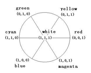
Figure 2. Decomposition of color (B, G, R)
It is coincident that only three items on the
right of equation (2) may be non-zero for a given color and the three cardinal
vectors or unique colors must be at the three vertexes of one of six sectors in
Figure 2. Hence equation (2) can be changed into
![]() (3)
(3)
where e1, e2
are two cardinal vectors or unique colors and m1, m2
are corresponding coefficients or magnitude of output codes.
Suppose
the angles at which e1 and e2 are located
(see Figure 2) are H1 and H2. Let
 ��4��
��4��
Then H, C, V, S will
represent hue, colorfulness, brightness, and saturation of (B, G, R)
properly if B, G and R are obtained from appropriate linear and nonlinear
transforms of spectral tri-stimulus values X, Y, Z (Lu, 1989). According
to the decoding model, the relation between brightness, colorfulness,
whiteness, blackness and B, G and R is shown in Figure 3, where
med(B, G, R) is the medium one or second one of B, G and R.
For example, med(1,3,5)=3, med(1,2,5)=2, med(1,5,5)=5, med(1,1,5)=1.
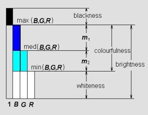
Figure 3 Relation between B, G, R and brightness,
colorfulness, whiteness, and blackness
Recently, I found the above
transform has been proposed earlier by A. R. Smith (1978), and introduced by
many scholars for computer graphics (J.D. Foley, A. Van Dam, 1984). The
detailed programs can be seen on web pages[1]
This shows that the decoding model is also practical. The different is that 1)B,
G, and R in A. R. Smith��s transform are the magnitudes of signals of
primary colors to stimulate a pixel of CRT instead of tri-stimulus values from
visual cones; 2)A. R. Smith used ��if-then�� programming language rather than
logical operations; 3)The following opponent process only exists in the
decoding model.
4. Opponent Process
We
use Venn's Diagram to show the essence of the process. Let ��,U,c denote the
three set operations: intersection, union, and complement respectively; B,
G, and R represent the three circular fields respectively (see
Figure 4). For convenience, we also use "-" for complement
operation and omit ��. Then, the eight fields can be represented by ![]() ,
, ![]() ,
, ![]() ,
, ![]() ,
, ![]() ,
, ![]() ,
, ![]() , and
, and ![]() .
.
Figure 4. Venn's diagram showing the logic of the opponent process
From
B, G and R, we can first get
![]() (5)
(5)
which represents the trefoil
(the intersecting fields of two or three of B, G, and R). Then,
we have
 (blue area)
(6)
(blue area)
(6)
where DeMorgan Law is used.
Similarly, there are
![]() (yellow area)
(7)
(yellow area)
(7)
![]() (green area)
(8)
(green area)
(8)
![]() (magenta area)
(9)
(magenta area)
(9)
![]() (red area)
(10)
(red area)
(10)
![]() (cyan area)
(11)
(cyan area)
(11)
Now
let B, G and R denote three receptor outputs and take values in
the set [0, 1], and the set operations be replaced by the fuzzy logic
operations: V, ��, - (V stands for maximum, �� for minimum and �C can be omitted). First we obtain the
medium one of B, G, and R (see Figure 5):
![]() (12)
(12)
Then we get three opponent
signals, blueness-yellowness (![]() ), greenness-magentaness (
), greenness-magentaness (![]() ), and redness-cyanness (
), and redness-cyanness (![]() ).The calculation as follows are surprisingly simple:
).The calculation as follows are surprisingly simple:
 (13)
(13)
 (14)
(14)
 (15)
(15)
The
opponent process corresponding to different monochromatic lights is shown in
Figure 5, where for convenience the three response curves are assumed. We can
also consider the left-upper part of Figure 5 as a Venn's diagram. There are
eight divided fields. The length of the part of a vertical line on a field is
just the magnitude of the corresponding unique color signal. These fields can
illustrate the change of color perception caused by different monochromatic
lights well.
Figure 5: Opponent process corresponding to
different monochromatic lights
5. Physical Model��
The
diagram of the principle of the opponent process in the decoding model is shown
in Figure 6.
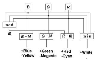
Figure 6. Symmetrically opponent process in the decoding model
In
order to demonstrate the process of color signals both in the retina and in the
cortex, I built a completely physical model of color vision (see Figure 7),
which works as well as I had expected.
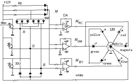
Figure 7. Diagram of principle of the physical model of color vision
Here
3DU is a phototransistor, which imitates a cone; DA is a differential
amplifier, which imitates a bipolar; LED is a light emitting diode, which is
assumed to be color cells in cortex; RE is a resister and 2DK is a diode. The
array of diodes and resisters on the upper left is assumed to be a horizontal
cell and provides output M=med(B,G,R).
The
physical model suggests that, in the cortex, there be seven color cells, which
receive white and six unique color signals; the brain produce brightness and
colorfulness by simple addition, and turns out hue and saturation by the
weighing method. Perhaps there are also some processes of color signals on
lower levels in retina. For example, some white cells probably receive faster
conducting signals directly from cones and rods (Kaplan, 1982). The decoding
model does not cover this subject. Thus, it does not provide a measure as
luminance Y in CIE XYZ or light value V in the Munsell system,
but V for brightness. The process of spatial information is also not
considered in the decoding model.
6. The Evolution of Color Vision��
According
to the decoding model, we can easily explain the evolution of color vision by
splitting sensitivity curves of visual cones (see Figure 8). Please imagine
that curves R(��) and G(��) gradually approach one
another to become one curve named Y(��). Then we would see the
fields representing red, green, cyan, and magenta disappear gradually. Further,
let curves B(��) and Y(��) approach one another gradually to become one curve
named W(��). Then we would see the fields representing blue and yellow disappear
gradually and only the black and white fields remain. Now, we can imagine that
color vision was evolving in the opposite procedure. First, there was only one
kind of visual cones in the human retina and only two totally different colors
(black and white) could be discerned. Then, with color vision evolving, the
cones split into two kinds that had different spectral sensitivities so that
blue and yellow were also perceived. After that, the cones split into three
kinds so that more colors were perceived.
Figure 8. Evolution of color vision illustrated by splitting
sensitivity curves
We
may conclude that n different kinds of cones can produce 2n
totally different color perceptions for n=1, 2, 3. As n=4, the
conclusion seems also true. We have built a symmetrical model of four primary
colors for robots (Lu, 1987). The model has 14 "unique colors", which
can be symmetrically put on the surface of a ball, besides "white"
(1, 1, 1, 1) and "black" (0, 0, 0, 0). We can get a "color"
ball that has many properties very similar to those in the Newton color wheel.
The
evolution of color vision might have come through somewhat different way. For
example (see Fig. 9, deuteranopia-2), the curve W(��) first split into R(��) and C(��) related to cyan, instead
of B(��) and Y(��), then C(��) split into B(��) and G(��).
7. Color Blindness��
Color
blindness has been discussed by many researchers (Hsia at el., 1965). It can
also be easily explained by the sensitivity curves of cones that are too close
each other. For example, monochromatism can be explained by the assumption that
the sensitivity curves B(��), G(��) and R(��) have not yet separated
from one curve; Red-green blindness can be explained by the assumption that the
curves G(��) and R(��) have not separated yet.
Figure 9 Different kinds of color blindness illustrated by incomplete separations
of three sensitive curves
According
to the decoding model, some red-green blindness can be identified as protanopia
or deuteranopia only because the peak of Y(��) has shorter or longer
wavelength. Tritanopia and tetartanopia can be illustrated by the assumption
that the B(��) and G(��) ( or B(��) and R(��) ) have not separated yet
so that each kind of color blindness can only perceive two chromatic colors:
red and cyan (or green and magenta). All kinds of color blindness above can be
imitated by the physical model with two of three of the 3DUs always obtain the
same light inputs.
Assuming
curve G(��) is split from the right curve or the left curve, we will have
different deuteranopia: deuteranopia-1 and deuteranopia-2, which produce
totally different color perceptions. However, according to philosophical
analyses about the inverted spectrum, two kinds of color blindness must be
equivalent and cannot be distinguished (Shoemaker, 1982; Lu, 1989).
Color
anomalous can be explained in similar way.
8. Discussion
There are many reasons that make
the decoding model convincible:
1)The
model is concise, symmetrical, and without modification parameters.
2)It
can more pictorially explain opponent process, color evolution, and color
blindness.
3)In
the popular zone model, adding red and green at the zone of visual cones forms
yellow; yet, adding red and green at the zone of visual nerves forms white. So,
meanings of ��red�� and ��green�� in popular zone model are inconsistent. Yet, the
decoding model has no this problem.
3)The
decoding model is more compatible with the laws of color mixture that are used
for color TV and computer graphics.
4)We
can also use the decoding model to explain the phenomenon of negative
after-image conveniently. For example, when the sensitivity of the R-cone
falls down, ![]() for cyanness
will be over zero for a white color (1,1,1) so that white color looks cyan.
for cyanness
will be over zero for a white color (1,1,1) so that white color looks cyan.
There
is seemingly also a problem with the decoding model. In the popular zone model,
there are only two pairs, instead of three pairs, of opponent colors. Seemingly
psychological and physiological experiments support the affirmation that only
two pairs of opponent colors exist. But, I think that the ��red and green�� in
popular zone model is actually a pair of opponent colors between red-cyan and
green-magenta. More than four unique colors were also affirmed by others
(Hardin, C. L., 1985).
According
to the decoding model, we can make two predictions. One is that there should be
some fuzzy logic gates, which execute the operations of maximum, minimum, and
even medium, in the human retina. Another is that there should be some
chromatic opponent units in visual nerves, whose response curves have a
horizontal line, instead of a neutral point, between positive and negative
parts (see the right part of figure 5). These logic gates and opponent units
have not been mentioned yet (which is another problem with the decoding model)
either because most experiments were made with animals whose color vision is
less complete than the man's, or because the guidance from appropriate theory
was absent. For example, a widely used method for identifying a chromatic
opponent unit is to find its neutral point (Volois and others, 1966); however,
this method is not suitable for identifying the opponent unit suggested above.
We believe that the predicted logic gates and the opponent units will be
discovered soon by physiologists who pay attention to them.
References
De Monasterio, F. M., Gouras P. and Tollhurst
D J., (1975) Trichromatic color opponency in ganglion cells of therhesus monkey
retina, J. Physiol. 252, 197-216
De Valois, Russell L.; Abramov, Israel; and Jacobs, Gerald H. (1966), "Analysis of response patterns of LGN cells", Journal of the Optical Society of America, 56(7): 966-977
Hardin, C. L.(1985) The resemblances of colors,
Philosophical Studies 48, 35-47
Hsia, Y. and Grapham, C. H., (1965) Color
blindness, in Visual Perception , C. H. Grapham ed., Wiley, New York, Chap. 14,
Tab.14.2
Hunt, R. W. G., (1982) A model of color vision for
predicting color appearance, Color Res. Appl. 7, 95-112
Hurvich, L. M. and Jameson D., (1957) An
opponent-process theory of color vision, Psychological Review 64, 384-404
James D. Foley, Andries Van Dam, (1984) Title
Fundamentals of Interactive Computer Graphics, Addison-Wesley
Judd, D. B., (1949) Response functions for
types of vision according to the Muller theory, J. Res. Natl. Bur. Std. 42
Kaplan, E. and Shapley, (1982) R. M., X and Y
cells in the lateral geniculale nucleus of Macaque monkeys, J. Physiol. 330,
125-143
Lu, C., (1986) New Theory of color vision and
simulation of mechanism, Developments in Psychology (in China), 14, 36-45
Lu, C., (1987) Models of color vision for
robots. Robot( A Journal of Chinese Society of Automation) , 1, No.6,39-46.
Lu, C., (1989) Decoding model and its
verification, ACTA OPTICA SINICA, 9, 158-163
Lu, C., (1989a) Clarifying ostensible
definition by the logical possibility of inverted spectrum, Modern Philosophy,
No.2, 1989
Lu, C., (1991) B-Fuzzy set algebra and
generalized mutual information formula, Fuzzy Systems and Mathematics, Vol. 5,
No. 1, 76-80
Lu, C., (1999) A generalization of Shannon's
information theory, Int. J. of General Systems, 28: (6) 453-490
Shoemaker S. (1982) The inverted spectrum��J��of Philosophy 79, 375-381
Smith, A. R.,(1978) Color Gamut Transform Pairs, Computer Graphics, Vol 12,
No 3, 12-19
Walraven, P. L., (1961) On the
Bezold-Brucke phenomenon, J. Opt. Soc. Am. 51, 1113-1116