Fisher information

From Wikipedia, the free encyclopedia

In statistics and information theory, the Fisher information (denoted $\mathcal{I}(\theta)$ ) is the variance of the score. It is named in honor of its inventor, the statistician R.A. Fisher.

[hide]

1 Definition
- 1.1 Single-parameter Bernoulli experiment
2 Matrix form
- 2.1 Multivariate normal distribution
3 See also

[edit] Definition

The Fisher information is the amount of information that an observable random variable X carries about an unknown parameter θ upon which the likelihood function of X, L(θ) = f(X; θ), depends. The likelihood function is the joint probability of the data, the Xs, conditional on the value of θ, as a function of θ. Since the expectation of the score is zero, the variance is simply the second moment of the score, the derivative of the log of the likelihood function with respect to θ. Hence the Fisher information can be written

$\mathcal{I}(\theta) = \mathrm{E} \left\{\left. \left[ \frac{\partial}{\partial\theta} \ln f(X;\theta) \right]^2 \right|\theta\right\},$

which implies $0 \leq \mathcal{I}(\theta) < \infty$ . The Fisher information is thus the expectation of the squared score. A random variable carrying high Fisher information implies that the absolute value of the score is often high.

The Fisher information is not a function of a particular observation, as the random variable X has been averaged out. The concept of information is useful when comparing two methods of observing a given random process.

If the following regularity condition is met:

$\int \frac{\partial^2}{\partial \theta^2}f(X ; \theta ) \, dx = 0,$

then the Fisher information may also be written as:

$\mathcal{I}(\theta) = - \mathrm{E} \left[ \frac{\partial^2}{\partial\theta^2} \ln f(X;\theta) \right].$

Thus Fisher information is the negative of the expectation of the second derivative of the log of f with respect to θ. Information may thus be seen to be a measure of the "sharpness" of the support curve near the maximum likelihood estimate of θ. A "blunt" support curve (one with a shallow maximum) would have a low expected second derivative, and thus low information; while a sharp one would have a high expected second derivative and thus high information.

Information is additive, in that the information yielded by two independent experiments is the sum of the information from each experiment separately:

$\mathcal{I}_{X,Y}(\theta) = \mathcal{I}_X(\theta) + \mathcal{I}_Y(\theta).$

This result follows from the elementary fact that if random variables are independent, the variance of their sum is the sum of their variances. Hence the information in a random sample of size n is n times that in a sample of size 1 (if observations are independent).

The information provided by a sufficient statistic is the same as that of the sample X. This may be seen by using Neyman's factorization criterion for a sufficient statistic. If T(X) is sufficient for θ, then

$f (X;θ) = g (T (X),θ) h (X)$

for some functions g and h. See sufficient statistic for a more detailed explanation. The equality of information then follows from the following fact:

$\frac{\partial}{\partial\theta} \ln \left[f(X ;\theta)\right] = \frac{\partial}{\partial\theta} \ln \left[g(T(X);\theta)\right]$

which follows from the definition of Fisher information, and the independence of h(X) from θ. More generally, if T = t(X) is a statistic, then

$\mathcal{I}_T(\theta) \leq \mathcal{I}_X(\theta)$

with equality if and only if T is a sufficient statistic.

The Cramér-Rao inequality states that the inverse of the Fisher information is an asymptotic lower bound on the variance of any unbiased estimator of θ.

Given a likelihood with $p$ parameters, we say that two parameters $θ i$ and $θ j$ are orthogonal if the element of the i-th row and j-th column of the Fisher Information is zero. Orthogonal parameters are easy to deal with in the sense that their maximum likelihood estimates are independent and can be calculated separately. When dealing with research problems, it is very common for the researcher to invest some time searching for an orthogonal parametrization of the densities involved in the problem.

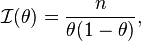
[edit] Single-parameter Bernoulli experiment

A Bernoulli trial is a random variable with two possible outcomes, "success" and "failure", with "success" having a probability of $θ$ . The outcome can be thought of as determined by a coin toss, with the probability of obtaining a "head" being $θ$ and the probability of obtaining a "tail" being $1 - θ$ .

The Fisher information contained in n independent Bernoulli trials may be calculated as follows. In the following, A represents the number of successes, B the number of failures, and n = A + B is the total number of trials.

$\mathcal{I}(\theta) = -\mathrm{E} \left[ \frac{\partial^2}{\partial\theta^2} \ln(f(A;\theta)) \right] \qquad (1)$

$= -\mathrm{E} \left[ \frac{\partial^2}{\partial\theta^2} \ln \left[ \theta^A(1-\theta)^B\frac{(A+B)!}{A!B!} \right] \right] \qquad (2)$

$= -\mathrm{E} \left[ \frac{\partial^2}{\partial\theta^2} \left[ A \ln (\theta) + B \ln(1-\theta) \right] \right] \qquad (3)$

$= -\mathrm{E} \left[ \frac{\partial}{\partial\theta} \left[ \frac{A}{\theta} - \frac{B}{1-\theta} \right] \right]$ (on differentiating ln x, see logarithm) $\qquad (4)$

$= +\mathrm{E} \left[ \frac{A}{\theta^2} + \frac{B}{(1-\theta)^2} \right] \qquad (5)$

$= \frac{n\theta}{\theta^2} + \frac{n(1-\theta)}{(1-\theta)^2}$ (as the expected value of $A = n θ$ , etc.) (6)

$= \frac{n}{\theta(1-\theta)} \qquad (7)$

(1) defines Fisher information. (2) invokes the fact that the information in a sufficient statistic is the same as that of the sample itself. (3) expands the log term and drops a constant. (4) and (5) differentiate with respect to $θ$ . (6) replaces A and B with their expectations. (7) is algebra.

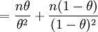
The end result, namely,

$\mathcal{I}(\theta) = \frac{n}{\theta(1-\theta)},$

is the reciprocal of the variance of the mean number of successes in n Bernoulli trials, as expected (see last sentence of the preceding section).

[edit] Matrix form

When there are N parameters, so that θ is a Nx1 vector $\theta = \begin{bmatrix} \theta_{1}, \theta_{2}, \cdots , \theta_{N} \end{bmatrix},$ , then the Fisher information takes the form of an NxN matrix, the Fisher information matrix (FIM), with typical element:

${\left(\mathcal{I} \left(\theta \right) \right)}_{i, j} = \mathrm{E} \left[ \frac{\partial}{\partial\theta_i} \ln f(X;\theta) \frac{\partial}{\partial\theta_j} \ln f(X;\theta) \right].$

The FIM is a NxN positive definite symmetric matrix, defining a metric on the N-dimensional parameter space. Exploring this topic requires differential geometry.

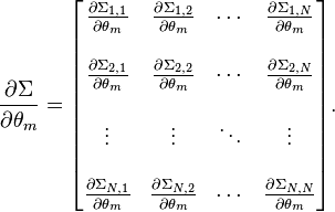
[edit] Multivariate normal distribution

The FIM for a N-variate multivariate normal distribution has a special form. Let $\mu(\theta) = \begin{bmatrix} \mu_{1}(\theta), \mu_{2}(\theta), \cdots , \mu_{N}(\theta) \end{bmatrix},$ and let $Σ(θ)$ be the covariance matrix of $μ(θ)$ . Then the typical element $\mathcal{I}_{m,n}$ , 0≤m,n<N, of the FIM for $X \sim N(\mu(\theta), \Sigma(\theta))$ is:

$\mathcal{I}_{m,n} = \frac{\partial \mu}{\partial \theta_m} \Sigma^{-1} \frac{\partial \mu^\top}{\partial \theta_n} + \frac{1}{2} \mathrm{tr} \left( \Sigma^{-1} \frac{\partial \Sigma}{\partial \theta_m} \Sigma^{-1} \frac{\partial \Sigma}{\partial \theta_n} \right),$

where $(..)^\top$ denotes the transpose of a vector, $tr(..)$ denotes the trace of a square matrix, and:

$\frac{\partial \mu}{\partial \theta_m} = \begin{bmatrix} \frac{\partial \mu_1}{\partial \theta_m} & \frac{\partial \mu_2}{\partial \theta_m} & \cdots & \frac{\partial \mu_N}{\partial \theta_m} & \end{bmatrix};$

$\frac{\partial \Sigma}{\partial \theta_m} = \begin{bmatrix} \frac{\partial \Sigma_{1,1}}{\partial \theta_m} & \frac{\partial \Sigma_{1,2}}{\partial \theta_m} & \cdots & \frac{\partial \Sigma_{1,N}}{\partial \theta_m} \\ \\ \frac{\partial \Sigma_{2,1}}{\partial \theta_m} & \frac{\partial \Sigma_{2,2}}{\partial \theta_m} & \cdots & \frac{\partial \Sigma_{2,N}}{\partial \theta_m} \\ \\ \vdots & \vdots & \ddots & \vdots \\ \\ \frac{\partial \Sigma_{N,1}}{\partial \theta_m} & \frac{\partial \Sigma_{N,2}}{\partial \theta_m} & \cdots & \frac{\partial \Sigma_{N,N}}{\partial \theta_m} \end{bmatrix}.$